Heat Transfer Today

Educational Software for
Heat and Mass Transfer

To assist engineering students in understanding the
fundamentals of heat and mass transfer while
exposing them to modern computational,
visualization and design techniques.

2004 ASME Curriculum Innovation Awards

Introduction

In the past most instructional-software packages for heat & mass transfer were based on the “computerization” of existing analytical solutions and experimental correlations. Often the result was a facility for doing more conventional calculations, only faster; and usually the computed result was just a single “answer” — such as an overall convective heat-transfer coefficient or fin efficiency.

By contrast, our software uses modern numerical algorithms to solve the fundamental governing ordinary or partial-differential equations in real time.  By combining this more fundamental approach with enhanced color-visualization techniques, these software modules allow a student to “see” — and thus perhaps to understand — the physics underlying a particular process.

We have developed software modules for ten (10) fundamental topics in heat transfer. About thirty (30) “mini-modules,” which use a combination of an Excel spreadsheet for input and graphical display of output and Visual Basic for Applications (VBA) macros for the serious calculations, have also been developed and may be downloaded here.

General Background

The algorithms and interfaces for each module are uniquely tailored for the particular application – thus avoiding the frequently-steep learning curves associated with much more powerful, commercially available and often costly CFD packages.  In most cases specific techniques were derived from the authors’ research, as well as from experience in graduate and undergraduate teaching.  All modules were used extensively for the first time by some sixty university students taking undergraduate Heat and Mass Transfer during the Spring 1996 semester and then sixteen more times in the Spring 1997-2013 semesters. All modules have been enhanced continuously and extensively as a result of these experiences.

Many of the original Fortran programs were developed and used as lecture demonstrations in distance education courses in Computational Fluid Dynamics and Heat Transfer taught through the Virginia Commonwealth Graduate Engineering Program.

Early Years in the Broadcast Studio

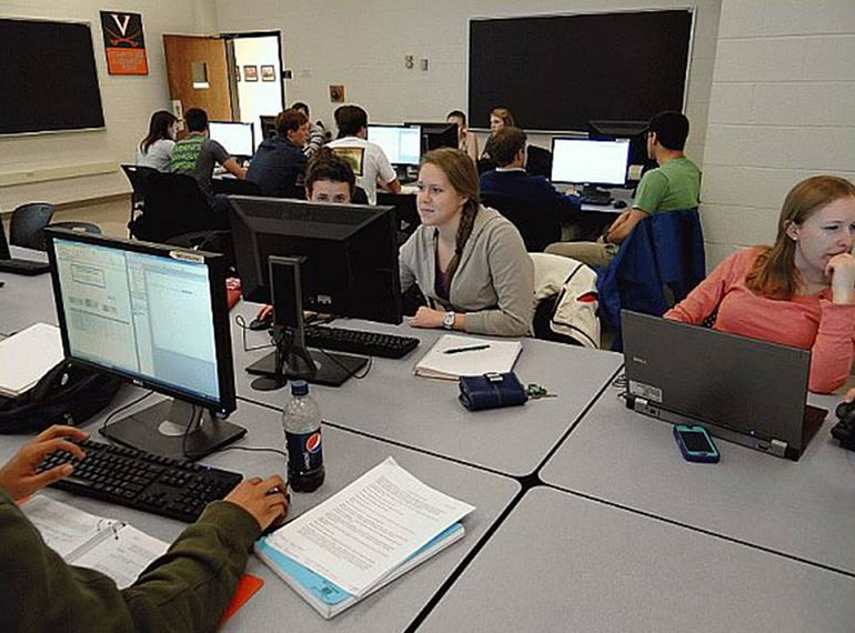
Then as facilities became available, they were used in a similar mode for a number of years in a projector-equipped, local classroom. The development of the graphical-user-interfaces during the 1995-96 academic year made them appropriate for student use as well, both on their own, or as we use them, in a scheduled “studio session.”  Students attend two 50-minute-long, traditional classes a week, but also have a two-hour working session in one of our computer classrooms.

Two-person Teams Working in the Studio Session

Originally Watcom Fortran 77 was used for the intense numerical computations and for generation of the color plots, while a tailored Visual Basic executable was used for the user interface.  Later all modules were ported to Visual Basic 6, allowing for much more interactivity than in the past.  At present all modules are written in VB 2013 and have been installed and tested in the “cloud.”

The development of the underlying computational routines, the user-interface, on-line help file, the supporting documentation, the student exercises, and in many cases a journal article is extremely time-consuming.  Consequently the topics for modules were chosen with great care.   Only fundamental subjects that cover at least ten pages in a typical textbook were selected.  In several cases virtually all the concepts from a whole chapter in a graduate-level text can be illustrated using one module. In addition, several of the modules are sufficiently general that they may be used in a variety of related courses, both graduate and undergraduate, in mathematics, science and engineering.

Contents/Site Map

Heat Transfer

For those looking for an entire software-enhanced introductory course in heat transfer, this table of contents is provided.   The chapter numbering is typical of several popular textbooks in the field.

1. Introduction to Heat Transfer

2. Conduction Fundamentals

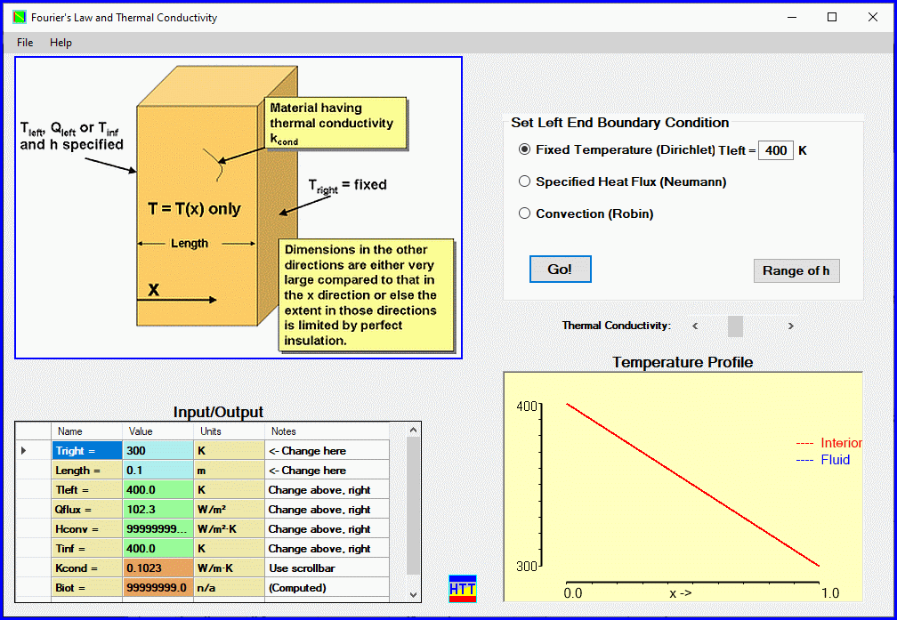
HTTFouriers.exe – Visual Studio module covering thermal conductivity and three types of thermal boundary conditions.

Airwater.xlsm – VBA Functions for properties of air and water as a function of temperature.

3. One-Dimensional, Steady-state Conduction

HTTextnd.exe – Visual Studio module for extended surface heat transfer (fins).

HTTtridiag.xlsm – 1-D, S-S conduction with generation in a plane wall.  Evaluates analytical solution as well as a finite-volume solution with linear equations solved (1) directly using Thomas algorithm and, (2) by iteration.

HTTnetwork.xlsm – Includes series and parallel lumped models for 1-D conduction.

HTTHeatedInsulation.xlsm – 1-D, steady-state heat-generating, insulated cylinder.

HTTFuelPin.xlsm – Simple model of temperature distribution in a nuclear fuel pin.

HTTBesselFunctions.xlsm – Analytical solution for efficiency of a straight, annular fin.

Project:  George Washington’s Compost Heap

Extra:   Extended Surface (Fin) Heat Transfer Photos

 4. Two-Dimensional, Steady-state Conduction

HTT_2dss.exe (Visual Studio module for 2-D, Steady-state Conduction)

Exercises – Workbook set up to record results from HTT_2dss module.

HTTtwodss.xlsm (Excel workbook demonstrating the evaluation and display of an analytical solution built up term-by-term for one particular 2-D, SS problem)

HTTiterdemos.xlsm (Excel workbook demonstrating iteration as a means of solving linear equations)

HTTConductionShapeFactors.xlsm (Excel workbook compilation of shape factors)

LinearEquations.xlsm (Excel workbook demonstrating both use of Excel’s supplied functions for solving linear equations and of a VBA subprogram for matrix inversion).

 5. Transient Conduction

HTTonedt.exe (Visual Studio module for 1-D, Transient Conduction (Burn your Heisler Charts!))

HTT_Cook.exe (Visual Studio module for Transient Conduction in a Finite-length Cylinder

HTTtransanal.xlsm (Excel workbook evaluating analytical (separation of variables) solution for transient conduction in plane wall)

HTTsemicalc.xlsm (Excel workbook for periodic conduction in a semi-infinite body)

Project: Monticello Transient Conduction Problem with a time-dependent convective boundary condition

Student Project: Transient Conduction at the Interface between Two Materials

Project: Sandwich Wall (ICF) Construction

Extra:  ICFHouse.pptx

Extra: Ground Source Heat Pump

6. Fundamentals of Convection

Extra:  Penguins.mp4 – Thermal Design and Family Life Issues in Emperor Penguins

7. External Forced Flow

HTTblasius.xlsm – Laminar flow over a heated flat plate using similarity method

HTTflatp.exe – Visual Studio virtual laboratory for laminar and turbulent flow over a flat plate

HTTBLCalcs.xlsm – Evaluate standard correlations for mixed convection over a flat plate and for a flat plate with unheated starting length

HTTtubeBanksZukauskas.xlsm – Empirical correlations for inline and staggered tube bundles.

Project: Convective Heat and Mass Transfer from a Runner

Project: Evaporative Cooling of Water in a Lister (Lyster) Bag.

Student Project:   Self-similar Boundary Layer Calculations

8. Internal Flows

HTT_pipe.exe – Visual Studio virtual laboratory for laminar and turbulent, thermal-entry-length flow

Corr_int.xlsm – Implementation of common correlations for internal flow forced convection. 

HTTRoughPipes.xlsm – Convection coefficients for rough pipes using the Colebrook equation for fluid mechanics with the Gnielinski correlation for heat transfer.

9. Natural Convection Flows

HTTncvfp.exe – Visual Studio virtual laboratory for natural convection adjacent to a vertical, flat plate calculated using classical similarity methods.

HTTporus.exe – Visual Studio virtual laboratory for natural convection in a saturated, permeable layer

10. Heat Transfer with Phase Change (Boiling and Condensation)

Extra: Trans-Alaska Pipeline Passive Cooling System

11.  Heat Exchangers

HTT_HX.exe – Visual Studio executable for design and performance calculations of “1-D” heat exchangers, i.e., simple parallel and counter-flow, shell-and-tube and parallel plate (first tab).  Design and performance calculations of “2-D” heat exchangers, i.e., cross-flow HX’s are on the 2nd tab.

HxEffectivenssNTU.xlsm – Effectiveness-NTU relations for a variety of HX geometries in algebraic, tabular, graphical and user-function forms. 

Extra:   Heat Exchanger Photos  

12. Radiation Fundamentals

HTTplnkslaw.xlsm – Calculation of blackbody emission spectrum and the blackbody integral as a function of temperature.

Project: Transmissivity of Glass

13. Radiative Exchange

HTTviewfactor.xlsm – This Excel workbook computes the view factors for four geometries for which analytical solutions are available and for which graphs are usually provided in textbooks.  Both display the input geometry to scale on the screen so that the user can check it carefully.  Another worksheet calculates the view factor between two arbitrarily-oriented parallelograms using a computer implementation of the Nusselt Unit-Sphere Method.

HTTRec2Rec.xlsm –  This workbook computes the view factor for rectangles in parallel planes and for rectangles in perpendicular planes.   Like the HTTviewfactor.xlsm workbook it draws the geometry to scale on the user’s screen so that they can check their inputs.   

HTTnetwork.xlsm – In addition to several examples using a DC network analogy for steady-state conduction, this spreadsheet includes several examples using the DC network analogy for gray body radiation.

HTTradiosity.xlsm – This Excel workbook provides a template for solving radiative exchange problems involving as many as 20 diffuse-gray surfaces exchanging heat among themselves.


Thermodynamics

Thermodynamic Properties

ProperT.xlsm – Properties of Fluids Using the free CoolProp Excel Add-in

MollierDiagram.xlsm – Mollier (Enthalpy-Entropy) Diagram

Extensive and Intensive Properties

Thermodynamic Processes

Filling and Emptying Tanks

Thermodynamic Cycles

Power Cycles

Otto (Spark Ignition) Cycle Template

Diesel (Compression Ignition) Cycle Template 

Brayton (Jet Engine) Cycle Template

Rankine Cycle Template

Humphrey Cycle Template

Ocean Thermal Energy Conversion (Rankine Cycle)

Refrigeration and Heat Pump Cycles

Vapor Compression Refrigeration Cycle

Residential Heat Pump in Winter 

Heat Pump Hot Water Heater

Extra: Ground Source Heat Pump

Fluid Mechanics

Aerodynamics

Wingtip Vortex Motion above a Runway 

Vortex Panel Method for a 2D Lifting Airfoil

Real Fluids 

Solution of Blasius Equation by Shooting

Compressible Flows

1D Compressible Flows (Isentropic flow with area change, normal shocks, Fanno line, Rayleigh line)

Oblique Planar Shocks

Computational Fluid Dynamics

Advection of a Passive Scalar in One and Two Dimensions

Elliptic Grid Generation for odd geometries

One-dimensional Wave Equation

Applications

1976 U.S. Standard Atmosphere

Velocity Triangles for Turbomachinery

Projectile Motion with Air Resistance Using 4th order Runge-Kutta


Highlights

  • Full-color visualization of fundamental concepts
  • Simple, straight-forward user-input – same as when using slide rules!
  • Graphical output emphasizing student insight
  • Thorough documentation, completely self-contained
  • Easy insertion into existing engineering curriculum
  • Virtual laboratories – perfect for online, active learning
  • Quality software – the programmer started programming in 1965
  • Classroom-tested and continuously improved for 17 years

System Requirements

  • Microsoft Windows
  • Intel-based PC
  • Screen resolution of at least 800×600
  • Mouse
  • Can be used with Mac and Unix in a virtualized environment

Software Modules for Heat Transfer

One-Dimensional, Transient Conduction (Heisler Charts!)

The mathematical description of transient heat conduction yields a second-order, parabolic, partial-differential equation. When applied to regular geometries such as infinite cylinders, spheres, and planar walls of small thickness, the equation simplifies to one having a single spatial dimension. With specification of an initial condition and two boundary conditions, the mathematician uses  separation of variables to solve the equation.   That process leads to an expression for temperature distribution in the form of an infinite series. The time-honored Heisler charts use a one-term approximation to the series and present the results in graphical form.  Heat transfer practitioners have used these charts widely for the last 75 years.

Module Description

The calculation In our software module, HTTonedt, we take a more fundamental numerical approach by computing a finite-volume (FVM) solution to the transient, one-dimensional heat equation.   We apply it to planar walls, infinite cylinders and spheres, i.e., the three geometries for which the Heisler Charts are used.  We use a single algorithm for all three, …

READ MORE

Transient Conduction in a Finite Cylinder (Cooking a Roast)

This module was intended for K-12 Outreach.  However, for the more advanced user it provides plenty of opportunities to learn the fundamentals of conduction heat transfer in solids. In it we model the cooking of a roast by solving the transient heat conduction equation in a finite, axisymmetric cylindrical geometry. The solution of the governing equation takes place entirely behind the scenes. The chef can “watch” the roast heat up over time. When cooking is completed, he or she can slice the roast at positions along its length and (virtually) sample the results.  The model includes both conventional “roasting” through heat transfer at its surface and volumetric heating as occurs in a microwave oven.

Module Description

ClickThis module includes a numerical solution (the finite-volume method) for the time-dependent, transient conduction equation in a homogeneous right circular cylinder. It assumes that during the heating and cooling process there are no chemical or physical changes in the material being cooked. Of course, in cooking a roast, there are both water migration and chemical …

READ MORE

Two-Dimensional, Steady-State Conduction

The mathematical description for multi-dimensional, steady-state heat-conduction is a second-order, elliptic partial-differential equation (a Laplace or Poisson Equation). Typical heat transfer textbooks describe several methods for solving this equation for two-dimensional regions with various boundary conditions. Analytical solutions usually involve an infinite series of transcendental functions. This series is truncated and evaluated at an array of locations to give an approximate estimate of the temperatures found over the 2-D region.  Some texts also include detailed graphical methods using various paper and pen tools for estimating temperature and heat-flow lines for 2-D problems.

Module Description

Inputs n our software module, HTT_2dss, we employ modern numerical methods.  Specifically the we use the finite-volume method, to solve for the temperature distribution over a user-specified 2-D region. The region is taken as rectangular, with cutouts possible. The user is asked to: specify the nodalization of the heat-conduction region.  We use dynamic array allocation, …

READ MORE

External Flows (Forced Convection over a Flat Plate)

In this module we model the boundary layer equations for forced convection over a flat plate in their primitive form.  That is, we relax the similarity restrictions of the Blasius solution. The result  can be considered a “virtual” laboratory.   The user can take the data produced in this simulation just as in a real physical laboratory.  But in this virtual laboratory they don’t need to worry about toxicity, burning themselves, etc.   Furthermore they can work with a range of fluids that no one physical laboratory could ever hope to study.

Module Description

InsightsInputs The user inputs the plate Reynolds and fluid Prandtl numbers, along with the freestream turbulence level (as a percent).  On a separate input form they may specify up to five independent zones where either the surface temperature or surface temperature gradient will be specified.  We use an algebraic model to estimate the transition point …

READ MORE

Internal Flows (Forced Convection in Pipes)

Internal Forced Flow (Pipe Flow)

Heat transfer analysts usually handle internal (pipe) flows using convection correlations. For laminar flows the correlations are based on analysis; for transition and turbulent flows they are generally based on experiment.  Another “on-screen” laboratory, our internal flow module instead solves the fundmental energy balance equation directly.    Here we address the thermal entry length problem.  In this scenario the velocity profile is already fully developed when a change in the wall thermal boundary condition is introduced.   Our model handles laminar, transition and turbulent flows.    The thermally (and hydrodynamically) fully developed condition is, of course, the asymptotic limit of the thermal entry problem.

The user of this “laboratory” selects either a fixed wall temperature or prescribed wall heat flux.  To solve the discretized form of the governing advection-diffusion equation, our algorithm uses a single pass, space-wise marching technique.  That scheme is implicit in the radial direction and is combined with backward differencing in the axial direction.

Module Description

Inputs Inputs to the model include the Prandtl number of the fluid, the Reynolds number based on diameter, the Length/Diameter ratio for the pipe.  The user selects whether a constant wall temperature or constant heat flux is applied to the surface. In addition, the user can specify a radial magnification factor for the display so …

READ MORE

Natural Convection in a Saturated Porous Layer

This module covers natural convection in a fluid-saturated, permeable material.  A number of recent graduate-level heat transfer texts cover this topic. The problem is analogous to classical Rayleigh-Benard natural convection in homogeneous fluid layers. The fluid is assumed to be “Boussinesq,” i.e., the fluid density is only a function of temperature and variable only in the body force term.  In addition, it completely fill all interstices.  The Darcy equations govern the fluid motion. Heating is from the bottom of the layer or from side to side.

Module Description

Inputs Before any run the user selects the aspect ratio of the layer and the number of grid points to be used in the vertical direction. The model uses the same grid spacing in both directions.  That being the case, we accomodate different aspect ratios by simply adding or subtracting columns of grid points in …

READ MORE

Analysis of Extended Surfaces (Fins and Heat Sinks)

The normal textbook treatment of heat transfer from fins involves the solution by analytical means of a single ordinary differential equation. That equation describes transport by conduction along the fin and convection from its surface. Even with a straight, rectangular fin, there is a quandary about what thermal boundary condition to apply at the tip.  Most practitioners resolve that question using an “extended length.”  In the case of straight fins of triangular cross-section and annular fins of constant thickness, the textbooks give  solutions in terms of Bessel functions, which the student may not have studied. Also, in the latter cases users never see the temperature distribution along the fin.  Graphical representation at best shows an overall (and confusing) parameter, the fin efficiency.   The major application of extended surface heat transfer is in arrays of fins (heat sinks.)

Module Description

Algorithm In this module we use a finite-volume solution of the governing heat balance equation instead.  The calculation includes terms representing conduction into and out of a short representative segment of the fin and convection from its surface.   We express the necessary derivatives of temperature in the conduction terms in terms of changes over small …

READ MORE

Heat Exchanger Design and Performance

The usual treatment of heat exchanger thermal design and analysis is based on two analysis-based solution methods applied to the governing, coupled heat balance equations.  For all but the simplest configurations, the solution of these differential equations by analytical means is challenging .   For this reason, the analytical results have been graphed in non-dimensional form.  Engineers have used the resulting charts routinely for the past three quarters of a century. The LMTD method is commonly used for heat exchanger design, that is, determining the required thermal size.   Similarly, the Effectiveness – NTU method is used for performance calculations.

Unfortunately, the charts and equations associated with these two methods do not give a complete picture of what is happening inside the exchanger, only a single overall measure. In this two-part module, our algorithm solves the same governing heat balance equations in real time in discretized form using modern numerical techniques.   The result is the same “bottom line” results as the traditional methods, but also a complete picture of what is happening within the device.  In addition, not having to look up a “correction factor” manually means the user can test parameters at will until an improved design is had.

Module Description

Introduction Our software for heat-exchanger education consists of a single module that covers both “1-D” and “2-D” exchangers: Use the first tab (algorithm) for double-pipe, shell-and-tube (with multiple shell passes) and 2-pass, 2-pass plate heat exchangers.  These configurations may be approximated as “one-dimensional”. Use the second tab (algorithm) for single-pass, crossflow heat-exchangers with the two …

READ MORE

Natural Convection next to a Heated, Vertical Flat Plate

This module solves the governing equations for natural convection next to a heated vertical flat plate in their similarity form.  We convert the continuity, vertical momentum (simplified using the Boussinesq approximation) and thermal energy equations into a pair of non-linear, coupled ordinary differential equations.  We specify the needed boundary conditions at both the surface of the plate and out at a distance from the plate.  We discretize the two equations and solve the resulting linear system iteratively.

Module Description

Inputs The only fluid input for the similarity solution is the Prandtl number of the fluid.  In addition, the user selects the extent of the computing region (ηmax) and the spatial increment (Δη) to be used.  Results in similarity form for vertical velocity and temperature are plotted in the left window.  The user supplies the …

READ MORE

Fourier’s Law, Conductivity and Boundary Conditions

This calculation allows the user to explore the effects of thermal boundary conditions and thermal conductivity in a simple, plane wall geometry. The user selects one of the three supplied thermal boundary conditions (fixed temperature (Dirichlet), specified heat flux (including the adiabatic condition) (Neumann) and convective boundary (Robin)), supplies numerical values of any parameters and performs the calculation. The resulting temperature distribution in the wall, computed using Fourier’s Law, is displayed.

Module Description

This module includes a library of typical materials, including photos and the corresponding magnitudes of the thermal conductivity.    Since the thermal conductivity can vary by a factor on the order of a million, dramatic differences in the solutions are readily apparent. Thermal conductivity form  

READ MORE
Web Design and SEO by

© 2021 Heat Transfer Today – All Rights Reserved.